Overview

In the first blog post of this series we have seen how we can represent words or tokens using Word2Vec. However, we also want representations that capture the context and meaning of words within different sentences.

A word in the context of one sentence might mean something different than the same word in another sentence. How can we capture that? Concepts like RNNs and LSTMs address this by preserving information about previous words in hidden state vectors. However, they have limitations such as vanishing gradient issues and computational inefficiency due to the need to compute all hidden states sequentially for a given sequence.

Generally, to overcome the limitation of models struggling to remember what they have already seen, such as earlier parts of a sentence, attention mechanisms are used. Attention introduces a direct connection between the prediction and relevant past information.

Self-attention goes a step further by allowing the model to relate each token to all other tokens in the sequence at once, moving away from strictly sequential processing of text.

Given a sentence such as “A cute teddy bear is reading”, to compute the representation of the word “teddy bear”, we need to consider all other tokens in the sequence simultaneously with direct connections. The representation of “teddy bear” becomes dependent on the full surrounding context.

The key concept behind self-attention is the Query (Q), Key (K), and Value (V) matrices.

Query, Key, and Value

The names sound abstract, so here is a simpler way to picture them. Think of self-attention as a soft lookup, a little like searching.

Every token asks a question: given what I am, which other tokens should I pay attention to? That question is the Query. Every token also advertises what it is about, like a label on a shelf. That label is the Key. And every token holds some actual content to pass on. That content is the Value.

To build the new representation of a token, we match its Query against the Key of every token in the sentence. Tokens whose Keys fit the Query well get a high score. We then pull in their Values, weighted by those scores. So a token ends up as a blend of the Values it found most relevant.

Building Q, K, and V

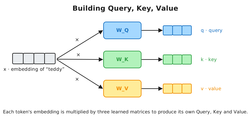
Where do Q, K, and V come from? We do not design them by hand. Each one is just the token embedding passed through a learned weight matrix.

For every token embedding x we compute:

q = x · W_Q     (Query)
k = x · W_K     (Key)
v = x · W_V     (Value)

W_Q, W_K, and W_V are three weight matrices that the model learns during training. They are shared across all tokens, so the same three matrices turn every embedding into its own q, k, and v.

In the original paper the embedding has size 512, and the q, k, v vectors have size 64.

Self-attention, step by step

Let us compute the new representation of one token, say “teddy”.

1. Score every pair

We take the Query q of “teddy” and compare it against the Key k of every token in the sentence, including “teddy” itself. The comparison is a dot product:

score_i = q · k_i

A large dot product means the two vectors point in a similar direction, so that token is relevant. A small one means it is not. After this step we have one score per token.

2. Scale

We divide every score by the square root of the key size, √d_k. With a key size of 64 that is a division by 8.

Why do this? When vectors are long, their dot products can get large. Large numbers push the next step (softmax) into a flat region where the gradients are tiny, and training becomes slow and unstable. Dividing by √d_k keeps the numbers in a sensible range. This is why the mechanism is called scaled dot-product attention.

3. Softmax

We pass the scaled scores through a softmax. Softmax turns a list of numbers into weights between 0 and 1 that add up to 1. You can read them as percentages: how much attention “teddy” pays to each token.

4. Weighted sum of Values

Finally we multiply each token’s Value by its weight and add them all up:

z = Σ weight_i · v_i

The result z is the new representation of “teddy”. It is no longer the plain embedding. It now carries information from the tokens it attended to.

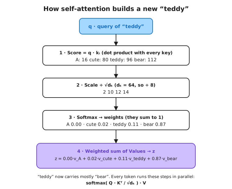
In the example above, “teddy” puts most of its weight on “bear”. That makes sense. To represent “teddy” well, the model needs to know it sits next to “bear”, so the new vector for “teddy” is mostly flavored by “bear”. This is exactly the context that plain Word2Vec embeddings could not give us.

Doing it all at once

We went token by token to keep things clear, but in practice we never loop. We stack all the queries into a matrix Q, all the keys into K, and all the values into V, and compute every token’s output in one go:

Attention(Q, K, V) = softmax( Q · Kᵀ / √d_k ) · V

That single line is the whole self-attention mechanism. Q · Kᵀ produces all the scores at once, √d_k scales them, softmax turns them into weights, and multiplying by V does the weighted sum. Because it is plain matrix multiplication, it runs fast on a GPU, and unlike an RNN it does not have to finish one step before starting the next.

Disadvantages of Transformers

Transformer architectures are efficient during training due to their ability to perform parallel computations across the input sequence. But dduring inference, the self-attention mechanism becomes computationally expensive because its complexity scales quadratically with the input length.

In self-attention, every token in a sequence is compared with every other token to determine how much attention it should pay to each one. Therefore, for a sequence with length L, the model needs to compute L × L attention scores, resulting in O(L²) computational complexity.

As the context window grows, the number of these comparisons increases rapidly. For example, doubling the sequence length does not double the computation required for self-attention, it increases it by a factor of four. This quadratic scaling makes Transformer models more expensive in terms of memory usage and inference latency when processing very long sequences.